


Computational complexity is a measure of how many resources are required to run an algorithm or solve a problem. It's a key field in computer science that helps programmers select and implement algorithms.
What does it measure?
- Time: How long it takes to run an algorithm
- Memory: How much memory is needed to run an algorithm
- Scalability: How well an algorithm scales as the number of inputs increases
How is it used?
- To predict how fast an algorithm will run
- To predict how much memory an algorithm will require
- To determine the practical limits of what computers can do
- To understand how computation time and space usage change as the size of an input changes
- To help us select the best algorithm based on input size
We use Big O Notation to describe the computational complexity of algorithms. Say we measure algorithm \(A\) and determine that based on the input size, \(n\), the time in milliseconds to run the algorithm takes \(t_A = 5n\). We have an alternate algorithm \(B\) that based on input size takes \(t_B = 0.1n^2\) milliseconds to run. Which algorithm should we choose?
Algorithm \(A\) seems to have a high coefficient whereas algorithm \(B\) the coefficient is a fraction of the one for \(A\). At \(n = 5\) we have \(t_A = 25\) and \(t_B = 2.5\). At \(n = 10\) we have \(t_A = 50\) and \(t_B = 10\). It seems that \(B\) is the better choice. But what happens when \(n\) gets much larger? At \(n = 100\) we have \(t_A = 500\) and \(t_B = 1000\). Now \(A\) appears to be the better choice. Using Big O analysis we could have easily figured this out without having to plug numbers into equations or even determining the exact form of the equations to start with.
The first algorithm exhibits linear behavior which is denoted in Big O notation as \(O(n)\). Notice that we use just the general form of the equation not the specific coefficients of an exact equation. Linear equations, \(y = 5x + 3\), \(y = 2x - 1\) and \(y = 10x\) are all represented by the same Big O notation \(O(n)\) used for linear forms. Likewise all quadratic forms such as \(y = 2x^2\), \(y = 5x^2 + 3x + 1\) or \(y = x^2 - 4\) are all represented by Big O notation \(O(n^2)\) as the dominant term when \(n\) gets large is the \(x^2\) term. Comparing the Big O forms \(O(n)\) to \(O(n^2)\) we can easily see that for large enough values of \(n\), algorithm \(B\) is always going to perform worse than \(A\) because quadratic \(O(n^2)\) forms always grow much faster than linear \(O(n)\) forms.
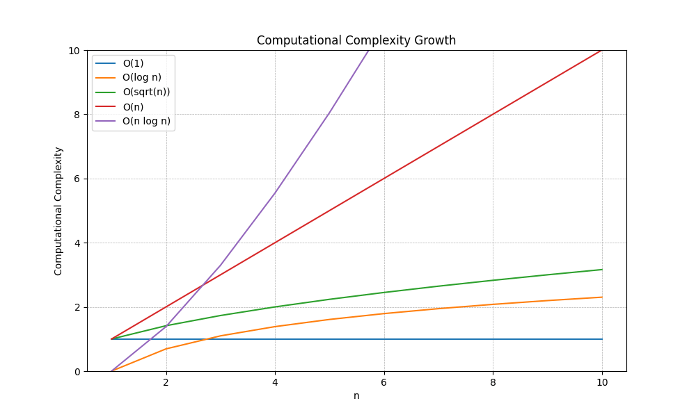
The graphs below illustrate the growth rate of common forms used in Big O notation. Even though for low values of \(n\) some algorithms may be better than others it is at large values of \(n\) that we are most concerned because it determines how much input data that we can process with a reasonable amount of resources.
From the first graph below we can see that constant time algorithms \(O(1)\) are always going to be the best. An example of a constant time algorithm would be accessing an element of an array given an index into the array. No matter how large the array gets, accessing an element is always going to take the same amount of time. We can also see the \(O(log\;n)\) and \(O(\sqrt n)\) are going to be pretty good because they grow very slowly with \(n\). Linear, \(O(n)\) is one of the most common. An example of a linear algorithm is to process all the elements of an array. The larger the array, the more time it takes but because the processing of each element is constant, the task of processing the whole array grows proportionately to the size of the array. Algorithms that process or search through arrays and single for loops are all indicators of \(O(n)\) algorithms. Slightly worse performance is indicated by \(O(n\;log\;n)\) algorithms.
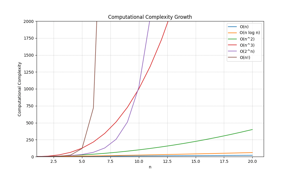
The second graph illustrates the growth rate of some very fast growing forms. \(O(n^2)\) is a common form as it can be descriptive of an algorithm that has one loop nested inside another. You can see that it grows at a much faster rate than linear algorithms. Even worse than polynomial forms \(O(n^2)\) and \(O(n^3)\) are the power forms like \(O(2^n)\). Perhaps the worst possible form is the factorial \(O(n!)\).
Knowing the hierarchy of Big O forms can help you to easily pick algorithms that have been characterized by Big O notation!
BigOPlot.py
import numpy as np
import matplotlib.pyplot as plt
import math

# Define n values
n = np.arange(1, 21)

# Define complexity functions
O_1 = np.ones_like(n)
O_log_n = np.log(n)
O_sqrt_n = np.sqrt(n)
O_n = n
O_n_log_N = n * np.log(n)
O_n2 = n**2
O_n3 = n**3
O_2n = 2**n
O_n_fact = np.array([math.factorial(i) for i in n])

# Plotting
plt.figure(figsize=(10, 6))

#plt.plot(n, O_1, label="O(1)")
#plt.plot(n, O_log_n, label="O(log n)")
#plt.plot(n, O_sqrt_n, label="O(sqrt(n))")
plt.plot(n, O_n, label="O(n)")
plt.plot(n, O_n_log_N, label="O(n log n)")
plt.plot(n, O_n2, label="O(n^2)")
plt.plot(n, O_n3, label="O(n^3)")
plt.plot(n, O_2n, label="O(2^n)")
plt.plot(n, O_n_fact, label="O(n!)")

plt.xlim(1, 21)  # Set y-axis to linear scale from 0 to 100
#plt.ylim(0, 10)  # Set y-axis to linear scale from 0 to 10
plt.ylim(0, 2000)  # Set y-axis to linear scale from 0 to 100
#plt.yscale('log')  # Use log scale for better visualization
plt.xlabel("n")
plt.ylabel("Computational Complexity")
plt.title("Computational Complexity Growth")
plt.legend()
plt.grid(True, which="both", linestyle="--", linewidth=0.5)

# Show the plot
plt.show()